In this tutorial, you will learn how to use Cyclical Learning Rates (CLR) and Keras to train your own neural networks. Using Cyclical Learning Rates you can dramatically reduce the number of experiments required to tune and find an optimal learning rate for your model.
Today is part two in our three-part series on tuning learning rates for deep neural networks:
- Part #1: Keras learning rate schedules and decay (last week’s post)
- Part #2: Cyclical Learning Rates with Keras and Deep Learning (today’s post)
- Part #3: Automatically finding optimal learning rates (next week’s post)
Last week we discussed the concept of learning rate schedules and how we can decay and decrease our learning rate over time according to a set function (i.e., linear, polynomial, or step decrease).
However, there are two problems with basic learning rate schedules:
- We don’t know what the optimal initial learning rate is.
- Monotonically decreasing our learning rate may lead to our network getting “stuck” in plateaus of the loss landscape.
Cyclical Learning Rates take a different approach. Using CLRs, we now:
- Define a minimum learning rate
- Define a maximum learning rate
- Allow the learning rate to cyclically oscillate between the two bounds
In practice, using Cyclical Learning Rates leads to faster convergence and with fewer experiments/hyperparameter updates.
And when we combine CLRs with next week’s technique on automatically finding optimal learning rates, you may never need to tune your learning rates again! (or at least run far fewer experiments to tune them).
To learn how to use Cyclical Learning Rates with Keras, just keep reading!
Looking for the source code to this post?
Jump right to the downloads section.
Cyclical Learning Rates with Keras and Deep Learning
In the first part of this tutorial, we’ll discuss Cyclical Learning Rates, including:
- What are Cyclical Learning Rates?
- Why should we use Cyclical Learning Rates?
- How do we use Cyclical Learning Rates with Keras?
From there, we’ll implement CLRs and train a variation of GoogLeNet on the CIFAR-10 dataset — I’ll even point out how to use Cyclical Learning Rates with your own custom datasets.
Finally, we’ll review the results of our experiments and you’ll see firsthand how CLRs can reduce the number of learning rate trials you need to perform to find an optimal learning rate range.
What are cyclical learning rates?
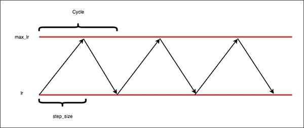
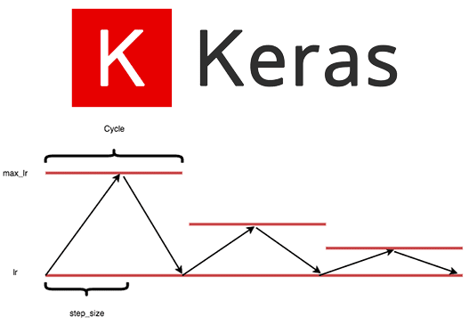
Figure 1: Cyclical learning rates oscillate back and forth between two bounds when training, slowly increasing the learning rate after every batch update. To implement cyclical learning rates with Keras, you simply need a callback.
As we discussed in last week’s post, we can define learning rate schedules that monotonically decrease our learning rate after each epoch.
By decreasing our learning rate over time we can allow our model to (ideally) descend into lower areas of the loss landscape.
In practice; however, there are a few problems with a monotonically decreasing learning rate:
- First, our model and optimizer are still sensitive to our initial choice in learning rate.
- Second, we don’t know what the initial learning rate should be — we may need to perform 10s to 100s of experiments just to find our initial learning rate.
- Finally, there is no guarantee that our model will descend into areas of low loss when lowering the learning rate.
To address these issues, Leslie Smith of the NRL introduced Cyclical Learning Rates in his 2015 paper, Cyclical Learning Rates for Training Neural Networks.
Now, instead of monotonically decreasing our learning rate, we instead:
- Define the lower bound on our learning rate (called “base_lr”).
- Define the upper bound on the learning rate (called the “max_lr”).
- Allow the learning rate to oscillate back and forth between these two bounds when training, slowly increasing and decreasing the learning rate after every batch update.
An example of a Cyclical Learning Rate can be seen in Figure 1.
Notice how our learning rate follows a triangular pattern. First, the learning rate is very small. Then, over time, the learning rate continues to grow until it hits the maximum value. The learning rate then descends back down to the base value. This cyclical pattern continues throughout training.
Why should we use Cyclical Learning Rates?
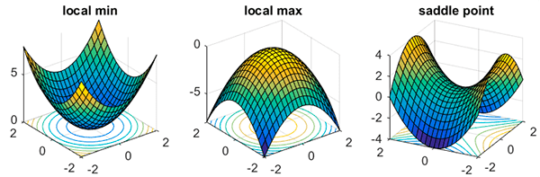
Figure 2: Monotonically decreasing learning rates could lead to a model that is stuck in saddle points or a local minima. By oscillating learning rates cyclically, we have more freedom in our initial learning rate, can break out of saddle points and local minima, and reduce learning rate tuning experimentation. (image source)
As mentioned above, Cyclical Learning Rates enables our learning rate to oscillate back and forth between a lower and upper bound.
So, why bother going through all the trouble?
Why not just monotonically decrease our learning rate, just as we’ve always done?
The first reason is that our network may become stuck in either saddle points or local minima, and the low learning rate may not be sufficient to break out of the area and descend into areas of the loss landscape with lower loss.
Secondly, our model and optimizer may be very sensitive to our initial learning rate choice. If we make a poor initial choice in learning rate, our model may be stuck from the very start.
Instead, we can use Cyclical Learning Rates to oscillate our learning rate between upper and lower bounds, enabling us to:
- Have more freedom in our initial learning rate choices.
- Break out of saddle points and local minima.
In practice, using CLRs leads to far fewer learning rate tuning experiments along with near identical accuracy to exhaustive hyperparameter tuning.
How do we use Cyclical Learning Rates?
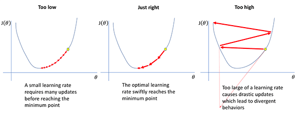
Figure 3: Brad Kenstler’s implementation of deep learning Cyclical Learning Rates for Keras includes three modes — “triangular”, “triangular2”, and “exp_range”. Cyclical learning rates seek to handle training issues when your learning rate is too high or too low shown in this figure. (image source)
We’ll be using Brad Kenstler’s implementation of Cyclical Learning Rates for Keras.
In order to use this implementation we need to define a few values first:
- Batch size: Number of training examples to use in a single forward and backward pass of the network during training.
- Batch/Iteration: Number of weight updates per epoch (i.e., # of total training examples divided by the batch size).
- Cycle: Number of iterations it takes for our learning rate to go from the lower bound, ascend to the upper bound, and then descend back to the lower bound again.
- Step size: Number of iterations in a half cycle. Leslie Smith, the creator of CLRs, recommends that the step_size should be
(2-8) * training_iterations_in_epoch
). In practice, I have found that step sizes or either 4 or 8 work well in most situations.
With these terms defined, let’s see how they work together to define a Cyclical Learning Rate policy.
The “triangular” policy
Figure 4: The “triangular” policy mode for deep learning cyclical learning rates with Keras.
The “triangular” Cyclical Learning Rate policy is a simple triangular cycle.
Our learning rate starts off at the base value and then starts to increase.
We reach the maximum learning rate value halfway through the cycle (i.e., the step size, or number of iterations in a half cycle). Once the maximum learning rate is hit, we then decrease the learning rate back to the base value. Again, it takes a half cycle to return to the base learning rate.
This entire process repeats (i.e., cyclical) until training is terminated.
The “triangular2” policy

Figure 5: The deep learning cyclical learning rate “triangular2” policy mode is similar to “triangular” but cuts the max learning rate bound in half after every cycle.
The “triangular2” CLR policy is similar to the standard “triangular” policy, but instead cuts our max learning rate bound in half after every cycle.
The argument here is that we get the best of both worlds:
We can oscillate our learning rate to break out of saddle points/local minima…
…and at the same time decrease our learning rate, enabling us to descend into lower loss areas of the loss landscape.
Furthermore, reducing our maximum learning rate over time helps stabilize our training. Later epochs with the “triangular” policy may exhibit large jumps in both loss and accuracy — the “triangular2” policy will help stabilize these jumps.
The “exp_range” policy
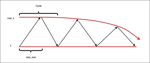
Figure 6: The “exp_range” cyclical learning rate policy undergoes exponential decay for the max learning rate bound while still exhibiting the “triangular” policy characteristics.
The “exp_range” Cyclical Learning Rate policy is similar to the “triangular2” policy, but, as the name suggests, instead follows an exponential decay, giving you more fine-tuned control in the rate of decline in max learning rate.
Note: In practice, I don’t use the “exp_range” policy — the “triangular” and “triangular2” policies are more than sufficient in the vast majority of projects.
How do I install Cyclical Learning Rates on my system?
The Cyclical Learning Rate implementation we are using is not pip-installable.
Instead, you can either:
- Use the “Downloads” section to grab the file and associated code/data for this tutorial.
- Download the
clr_callback.py
file from the GitHub repo (linked to above) and insert it into your project.
From there, let’s move on to training our first CNN using a Cyclical Learning Rate.
Project structure
Go ahead and run the
treecommand from within the
keras-cyclical-learning-rates/directory to print our project structure:
$ tree --dirsfirst
.
├── output
│   ├── triangular2_clr_plot.png
│   ├── triangular2_training_plot.png
│   ├── triangular_clr_plot.png
│   └── triangular_training_plot.png
├── pyimagesearch
│   ├── __init__.py
│   ├── clr_callback.py
│   ├── config.py
│   └── minigooglenet.py
└── train_cifar10.py

2 directories, 9 files
The
output/directory will contain our CLR and accuracy/loss plots.
The
pyimagesearchmodule contains our cyclical learning rate callback class, MiniGoogLeNet CNN, and configuration file:
- The
clr_callback.py
file contains the Cyclical Learning Rate callback which will update our learning rate automatically at the end of each batch update. - The
minigooglenet.py
file holds theMiniGoogLeNet
CNN which we will train using CIFAR-10 data. We will not review MiniGoogLeNet today — please refer to Deep Learning for Computer Vision with Python to learn more about this CNN architecture. - Our
config.py
is simply a Python file containing configuration variables — we’ll review it in the next section.
Our training script,
train_cifar10.py, trains MiniGoogLeNet using the CIFAR-10 dataset. The training script takes advantage of our CLR callback and configuration.
Our configuration file
Before we implement our training script, let’s first review our configuration file:
# import the necessary packages
import os

# initialize the list of class label names
CLASSES = ["airplane", "automobile", "bird", "cat", "deer", "dog",
	"frog", "horse", "ship", "truck"]
We will use the
osmodule in our config so that we can construct operating system-agnostic paths directly (Line 2).
From there, our CIFAR-10
CLASSESare defined (Lines 5 and 6).
Let’s define our cyclical learning rate parameters:
# define the minimum learning rate, maximum learning rate, batch size,
# step size, CLR method, and number of epochs
MIN_LR = 1e-7
MAX_LR = 1e-2
BATCH_SIZE = 64
STEP_SIZE = 8
CLR_METHOD = "triangular"
NUM_EPOCHS = 96
The
MIN_LRand
MAX_LRdefine our base learning rate and maximum learning rate, respectively (Lines 10 and 11). I know these learning rates will work well when training MiniGoogLeNet per the experiments I have already run for Deep Learning for Computer Vision with Python — next week I will show you how to automatically find these values.
The
BATCH_SIZE(Line 12) is the number of training examples per batch update.
We then have the
STEP_SIZEwhich is the number of batch updates in a half cycle (Line 13).
The
CLR_METHODcontrols our Cyclical Learning Rate policy (Line 14). Here we are using the
”triangular”policy, as discussed in the previous section.
We can calculate the number of full CLR cycles in a given number of epochs via:
NUM_CLR_CYCLES = NUM_EPOCHS / STEP_SIZE / 2
For example, with
NUM_EPOCHS = 96and
STEP_SIZE = 8, there will be a total of 6 full cycles:
96 / 8 / 2 = 6.
Finally, we define our output plot paths/filenames:
# define the path to the output training history plot and cyclical
# learning rate plot
TRAINING_PLOT_PATH = os.path.sep.join(["output", "training_plot.png"])
CLR_PLOT_PATH = os.path.sep.join(["output", "clr_plot.png"])
We’ll plot a training history accuracy/loss plot as well as a cyclical learning rate plot. You may specify the paths + filenames of the plots on Lines 19 and 20.
Implementing our Cyclical Learning Rate training script
With our configuration defined, we can move on to implementing our training script.
Open up
trian_cifar10.pyand insert the following code:
# set the matplotlib backend so figures can be saved in the background
import matplotlib
matplotlib.use("Agg")

# import the necessary packages
from pyimagesearch.minigooglenet import MiniGoogLeNet
from pyimagesearch.clr_callback import CyclicLR
from pyimagesearch import config
from sklearn.preprocessing import LabelBinarizer
from sklearn.metrics import classification_report
from keras.preprocessing.image import ImageDataGenerator
from keras.optimizers import SGD
from keras.datasets import cifar10
import matplotlib.pyplot as plt
import numpy as np
Lines 2-15 import our necessary packages. Most notably our
CyclicLR(from the
clr_callbackfile) is imported via Line 7. The
matplotlibbackend is set on Line 3 so that our plots can be written to disk at the end of the training process.
Next, let’s load our CIFAR-10 data:
# load the training and testing data, converting the images from
# integers to floats
print("[INFO] loading CIFAR-10 data...")
((trainX, trainY), (testX, testY)) = cifar10.load_data()
trainX = trainX.astype("float")
testX = testX.astype("float")

# apply mean subtraction to the data
mean = np.mean(trainX, axis=0)
trainX -= mean
testX -= mean

# convert the labels from integers to vectors
lb = LabelBinarizer()
trainY = lb.fit_transform(trainY)
testY = lb.transform(testY)

# construct the image generator for data augmentation
aug = ImageDataGenerator(width_shift_range=0.1,
	height_shift_range=0.1, horizontal_flip=True,
	fill_mode="nearest")
Lines 20-22 load the CIFAR-10 image dataset. The data is pre-split into training and testing sets.
From there, we calculate the
meanand apply mean subtraction (Lines 25-27). Mean subtraction is a normalization/scaling technique that results in improved model accuracy. For more details, please refer to the Practitioner Bundle of Deep Learning for Computer Vision with Python.
Labels are then binarized (Lines 30-32).
Next, we initialize our data augmentation object (Lines 35-37). Data augmentation increases model generalization by producing randomly mutated images from your dataset during training. I’ve written about data augmentation in-depth in Deep Learning for Computer Vision with Python as well as two blog posts (How to use Keras fit and fit_generator (a hands-on tutorial) and Keras ImageDataGenerator and Data Augmentation).
Let’s initialize (1) our model, and (2) our cyclical learning rate callback:
# initialize the optimizer and model
print("[INFO] compiling model...")
opt = SGD(lr=config.MIN_LR, momentum=0.9)
model = MiniGoogLeNet.build(width=32, height=32, depth=3, classes=10)
model.compile(loss="categorical_crossentropy", optimizer=opt,
	metrics=["accuracy"])

# initialize the cyclical learning rate callback
print("[INFO] using '{}' method".format(config.CLR_METHOD))
clr = CyclicLR(
	mode=config.CLR_METHOD,
	base_lr=config.MIN_LR,
	max_lr=config.MAX_LR,
	step_size= config.STEP_SIZE * (trainX.shape[0] // config.BATCH_SIZE))
Our
modelis initialized with stochastic gradient descent (
SGD) optimization and
"categorical_crossentropy"loss (Lines 41-44). If you have only two classes in your dataset, be sure to set
loss="binary_crossentropy".
Next, we initialize the cyclical learning rate callback via Lines 48-52. The CLR parameters are provided to the constructor. Now is a great time to review them at the top of the “How do we use Cyclical Learning Rates?” section above. The
step_sizefollow’s Leslie Smith’s recommendation of setting it to be a multiple of the number of batch updates per epoch.
Let’s train and evaluate our model using CLR now:
# train the network
print("[INFO] training network...")
H = model.fit_generator(
	aug.flow(trainX, trainY, batch_size=config.BATCH_SIZE),
	validation_data=(testX, testY),
	steps_per_epoch=trainX.shape[0] // config.BATCH_SIZE,
	epochs=config.NUM_EPOCHS,
	callbacks=[clr],
	verbose=1)

# evaluate the network and show a classification report
print("[INFO] evaluating network...")
predictions = model.predict(testX, batch_size=config.BATCH_SIZE)
print(classification_report(testY.argmax(axis=1),
	predictions.argmax(axis=1), target_names=config.CLASSES))
Lines 56-62 launch training using the
clrcallback and data augmentation.
Then Lines 66-68 evaluate the network on the testing set and print a
classification_report.
Finally, we’ll generate two plots:
# construct a plot that plots and saves the training history
N = np.arange(0, config.NUM_EPOCHS)
plt.style.use("ggplot")
plt.figure()
plt.plot(N, H.history["loss"], label="train_loss")
plt.plot(N, H.history["val_loss"], label="val_loss")
plt.plot(N, H.history["acc"], label="train_acc")
plt.plot(N, H.history["val_acc"], label="val_acc")
plt.title("Training Loss and Accuracy")
plt.xlabel("Epoch #")
plt.ylabel("Loss/Accuracy")
plt.legend(loc="lower left")
plt.savefig(config.TRAINING_PLOT_PATH)

# plot the learning rate history
N = np.arange(0, len(clr.history["lr"]))
plt.figure()
plt.plot(N, clr.history["lr"])
plt.title("Cyclical Learning Rate (CLR)")
plt.xlabel("Training Iterations")
plt.ylabel("Learning Rate")
plt.savefig(config.CLR_PLOT_PATH)
Two plots are generated:
- Training accuracy/loss history (Lines 71-82). The standard plot format included in most of my tutorials and every experiment of my deep learning book.
- Learning rate history (Lines 86-91). This plot will help us to visually verify that our learning rate is oscillating according to our intentions.
Training with cyclical learning rates
We are now ready to train our CNN using Cyclical Learning Rates with Keras!
Make sure you’ve used the “Downloads” section of this post to download the source code — from there, open up a terminal and execute the following command:
$ python train_cifar10.py
[INFO] loading CIFAR-10 data...
[INFO] compiling model...
[INFO] using 'triangular' method
[INFO] training network...
Epoch 1/96
781/781 [==============================] - 100s 128ms/step - loss: 1.9371 - acc: 0.2864 - val_loss: 1.5345 - val_acc: 0.4460
Epoch 2/96
781/781 [==============================] - 97s 124ms/step - loss: 1.3926 - acc: 0.4956 - val_loss: 1.3106 - val_acc: 0.5454
Epoch 3/96
781/781 [==============================] - 96s 123ms/step - loss: 1.1397 - acc: 0.5906 - val_loss: 1.1766 - val_acc: 0.5875
Epoch 4/96
781/781 [==============================] - 96s 123ms/step - loss: 0.9629 - acc: 0.6600 - val_loss: 0.8561 - val_acc: 0.7054
Epoch 5/96
781/781 [==============================] - 96s 123ms/step - loss: 0.8405 - acc: 0.7067 - val_loss: 0.9309 - val_acc: 0.6837
...
Epoch 92/96
781/781 [==============================] - 96s 123ms/step - loss: 0.0604 - acc: 0.9798 - val_loss: 0.3729 - val_acc: 0.9047
Epoch 93/96
781/781 [==============================] - 96s 123ms/step - loss: 0.0475 - acc: 0.9842 - val_loss: 0.3786 - val_acc: 0.9087
Epoch 94/96
781/781 [==============================] - 96s 122ms/step - loss: 0.0383 - acc: 0.9878 - val_loss: 0.3567 - val_acc: 0.9114
Epoch 95/96
781/781 [==============================] - 96s 123ms/step - loss: 0.0303 - acc: 0.9904 - val_loss: 0.3551 - val_acc: 0.9144
Epoch 96/96
781/781 [==============================] - 96s 123ms/step - loss: 0.0275 - acc: 0.9921 - val_loss: 0.3347 - val_acc: 0.9168
[INFO] evaluating network...
10000/10000 [==============================] - 5s 517us/step
              precision    recall  f1-score   support

    airplane       0.92      0.94      0.93      1000
  automobile       0.94      0.97      0.95      1000
        bird       0.88      0.89      0.89      1000
         cat       0.84      0.83      0.83      1000
        deer       0.92      0.92      0.92      1000
         dog       0.89      0.85      0.87      1000
        frog       0.92      0.95      0.93      1000
       horse       0.95      0.94      0.95      1000
        ship       0.95      0.95      0.95      1000
       truck       0.95      0.94      0.94      1000

   micro avg       0.92      0.92      0.92     10000
   macro avg       0.92      0.92      0.92     10000
weighted avg       0.92      0.92      0.92     10000
As you can see, by using the “triangular” CLR policy we are obtaining 92% accuracy on our CIFAR-10 testing set.
The following figure shows the learning rate plot, demonstrating how it cyclically starts at our lower learning rate bound, increases to the maximum value at half a cycle, and then decreases again to the lower bound, completing the cycle:

Figure 7: Our first experiment of deep learning cyclical learning rates with Keras uses the “triangular” policy.
Examining our training history you can see the cyclical behavior of the learning rate:
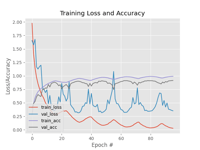
Figure 8: Our first experiment training history plot shows the effects of the “triangular” policy on the accuracy/loss curves.
Notice the “wave” in the training accuracy and validation accuracy — the bottom of the wave is our base learning rate, the top of the wave is the upper bound on the learning rate, and the bottom of the wave, just before the next one starts, is the lower learning rate.
Just for fun, go back to Line 14 of the
config.pyfile and update the
CLR_METHODto be
”triangular2”instead of
”triangular”:
# define the minimum learning rate, maximum learning rate, batch size,
# step size, CLR method, and number of epochs
MIN_LR = 1e-7
MAX_LR = 1e-2
BATCH_SIZE = 64
STEP_SIZE = 8
CLR_METHOD = "triangular2"
NUM_EPOCHS = 96
From there, train the network:
$ python train_cifar10.py
[INFO] loading CIFAR-10 data...
[INFO] compiling model...
[INFO] using 'triangular2' method
[INFO] training network...
Epoch 1/96
781/781 [==============================] - 100s 128ms/step - loss: 1.9570 - acc: 0.2773 - val_loss: 1.6161 - val_acc: 0.4176
Epoch 2/96
781/781 [==============================] - 96s 123ms/step - loss: 1.4089 - acc: 0.4848 - val_loss: 1.3741 - val_acc: 0.5182
Epoch 3/96
781/781 [==============================] - 96s 123ms/step - loss: 1.1591 - acc: 0.5876 - val_loss: 1.3593 - val_acc: 0.5570
Epoch 4/96
781/781 [==============================] - 96s 123ms/step - loss: 0.9897 - acc: 0.6520 - val_loss: 0.9174 - val_acc: 0.6727
Epoch 5/96
781/781 [==============================] - 96s 123ms/step - loss: 0.8656 - acc: 0.6985 - val_loss: 0.9247 - val_acc: 0.6855
...
Epoch 92/96
781/781 [==============================] - 96s 123ms/step - loss: 0.0715 - acc: 0.9766 - val_loss: 0.3728 - val_acc: 0.8963
Epoch 93/96
781/781 [==============================] - 96s 123ms/step - loss: 0.0692 - acc: 0.9772 - val_loss: 0.3744 - val_acc: 0.8957
Epoch 94/96
781/781 [==============================] - 96s 123ms/step - loss: 0.0707 - acc: 0.9770 - val_loss: 0.3689 - val_acc: 0.8959
Epoch 95/96
781/781 [==============================] - 96s 123ms/step - loss: 0.0694 - acc: 0.9780 - val_loss: 0.3685 - val_acc: 0.8972
Epoch 96/96
781/781 [==============================] - 96s 123ms/step - loss: 0.0687 - acc: 0.9773 - val_loss: 0.3708 - val_acc: 0.8978
[INFO] evaluating network...
10000/10000 [==============================] - 5s 520us/step
              precision    recall  f1-score   support

    airplane       0.90      0.92      0.91      1000
  automobile       0.94      0.96      0.95      1000
        bird       0.85      0.86      0.85      1000
         cat       0.82      0.79      0.80      1000
        deer       0.88      0.87      0.88      1000
         dog       0.85      0.84      0.85      1000
        frog       0.90      0.94      0.92      1000
       horse       0.94      0.92      0.93      1000
        ship       0.96      0.94      0.95      1000
       truck       0.93      0.94      0.94      1000

   micro avg       0.90      0.90      0.90     10000
   macro avg       0.90      0.90      0.90     10000
weighted avg       0.90      0.90      0.90     10000
This time we are obtaining 90% accuracy, slightly lower than using the “triangular” policy.
Our learning rate plot visualizes how our learning rate is cyclically updated:
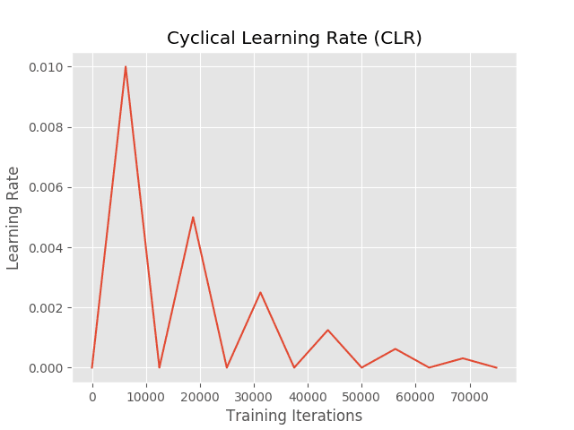
Figure 9: Our second experiment uses the “triangular2” cyclical learning rate policy mode. The actual learning rates throughout training are shown in the plot.
Notice at after each complete cycle the maximum learning rate is halved. Since our maximum learning rate is decreasing after every cycle, our “waves” in the training and validation accuracy will be much less pronounced:

Figure 10: Our second experiment training history plot shows the effects of the “triangular2” policy on the accuracy/loss curves.
While the “triangular” Cyclical Learning Rate policy obtained slightly better accuracy, it also exhibited far much fluctuation and had more risk of overfitting.
In contrast, the “triangular2” policy, while being less accurate, is more stable in its training.
When performing your own experiments with Cyclical Learning Rates I suggest you test both policies and choose the one that balances both accuracy and stability (i.e., stable training with less risk of overfitting).
In next week’s tutorial, I’ll show you how you can automatically define your minimum and maximum learning rate bounds with Cyclical Learning Rates.
Where can I learn more?
Figure 11: My deep learning book, Deep Learning for Computer Vision with Python, is trusted by employees and students of top institutions.
If you’re interested in diving head-first into the world of computer vision/deep learning and discovering how to:
- Train Convolutional Neural Networks on your own custom datasets
- Replicate the results of state-of-the-art papers, including ResNet, SqueezeNet, VGGNet, and others
- Train your own custom Faster R-CNN, Single Shot Detectors (SSDs), and RetinaNet object detectors
- Use Mask R-CNN to train your own instance segmentation networks
- Train Generative Adversarial Networks (GANs)
…then be sure to take a look at my book, Deep Learning for Computer Vision with Python!
My complete, self-study deep learning book is trusted by members of top machine learning schools, companies, and organizations, including Microsoft, Google, Stanford, MIT, CMU, and more!
Readers of my book have gone on to win Kaggle competitions, secure academic grants, and start careers in CV and DL using the knowledge they gained through study and practice.
My book not only teaches the fundamentals, but also teaches advanced techniques, best practices, and tools to ensure that you are armed with practical knowledge and proven coding recipes to tackle nearly any computer vision and deep learning problem presented to you in school, in your research, or in the modern workforce.
Be sure to take a look — and while you’re at it, don’t forget to grab your (free) table of contents + sample chapters.
Summary
In this tutorial, you learned how to use Cyclical Learning Rates (CLRs) with Keras.
Unlike standard learning rate decay schedules, which monotonically decrease our learning rate, CLRs instead:
- Define a minimum learning rate
- Define a maximum learning rate
- Allow the learning rate to cyclically oscillate between the two bounds
Cyclical Learning rates often lead to faster convergence with fewer experiments and hyperparameter tuning.
But there’s still a problem…
How do we know that the optimal lower and upper bounds of the learning rate are?
That’s a great question — and I’ll be answering it in next week’s post where I’ll show you how to automatically find optimal learning rate values.
I hope you enjoyed today’s post!
To download the source code to this post (and be notified when future tutorials are published here on PyImageSearch), just enter your email address in the form below.
Downloads:
The post Cyclical Learning Rates with Keras and Deep Learning appeared first on PyImageSearch.